5: Spatial Econometric Interaction Model

Author

Magdalene Chan

Published

December 16, 2023

Modified

December 16, 2023

Getting started

The key packages to be used in this exercise are:

tmap: for thematic mapping
sf: for geospatial data wrangling
spdep: for spatial weights matrix
spflow: for spatial econometric models of O-D flow
tidyverse: for non-spatial data wrangling

However, as the latest version of the spflow package is not available on CRAN yet, the install_github() function of devtools package will be used to install the spflow package first.

devtools::install_github("LukeCe/spflow")
# Check that version number should be at least 0.1.0.9010

The code chunk below then uses p_load() of pacman package to check if the required packages have been installed on the computer. If they are, the packages will be launched.

pacman::p_load(tmap, sf, spdep, sp, Matrix, spflow, knitr, tidyverse)

Data Preparation

Before calibrating Spatial Econometric Interaction Models using spflow, three data sets are required:

spatial weights
tibble data frame O-D flow matrix (with distance)
tibble data frame consisting of explanatory variables (does not need to differentiate origin vs. destination variables)

mpsz_nb <- read_rds("data/rds/mpsz_nb.rds")
mpsz_flow <- read_rds("data/rds/mpsz_flow.rds")
mpsz_var <- read_rds("data/rds/mpsz_var.rds")

Creating `spflow_network-class` objects

spflow_network-class is an S4 class containing information on a spatial network which is composed by a set of nodes that are linked by some neighbourhood relation. It can be created using spflow_network() function of spflow package. For our model, we choose the contiguity based neighbourhood structure.

mpsz_net <- spflow_network(
  id_net = "sg",  # assign an id name, can give it any input
  node_neighborhood = nb2mat(mpsz_nb$by_contiguity),
  node_data = mpsz_var,
  node_key_column = "SZ_CODE"
)

mpsz_net

Spatial network nodes with id: sg
--------------------------------------------------
Number of nodes: 313
Average number of links per node: 6.077
Density of the neighborhood matrix: 1.94% (non-zero connections)

Data on nodes:
                SZ_NAME SZ_CODE BUSSTOP_COUNT AGE7_12 AGE13_24 AGE25_64
1      INSTITUTION HILL  RVSZ05             2     330      360     2260
2        ROBERTSON QUAY  SRSZ01            10     320      350     2200
3          FORT CANNING  MUSZ02             6       0       10       30
4      MARINA EAST (MP)  MPSZ05             2       0        0        0
5               SENTOSA  SISZ01             1     200      260     1440
6        CITY TERMINALS  BMSZ17            10       0        0        0
---                 ---     ---           ---     ---      ---      ---
308            NEE SOON  YSSZ07            12      90      140      590
309       UPPER THOMSON  BSSZ01            47    1590     3660    15980
310          SHANGRI-LA  AMSZ05            12     810     1920     9650
311          TOWNSVILLE  AMSZ04             9     980     2000    11320
312           MARYMOUNT  BSSZ02            25    1610     4060    16860
313 TUAS VIEW EXTENSION  TSSZ06            11       0        0        0
    SCHOOL_COUNT BUSINESS_COUNT RETAILS_COUNT FINSERV_COUNT ENTERTN_COUNT
1              1              6            26             3             0
2              0              4           207            18             6
3              0              7            17             0             3
4              0              0             0             0             0
5              0              1            84            29             2
6              0             11            14             4             0
---          ---            ---           ---           ---           ---
308            0              0             7             0             0
309            3             21           305            30             0
310            3              0            53             9             0
311            1              0            83            11             0
312            3             19           135             8             0
313            0             53             3             1             0
    FB_COUNT LR_COUNT COORD_X COORD_Y
1          4        3  103.84    1.29
2         38       11  103.84    1.29
3          4        7  103.85    1.29
4          0        0  103.88    1.29
5         38       20  103.83    1.25
6         15        0  103.85    1.26
---      ---      ---     ---     ---
308        0        0  103.81     1.4
309        5       11  103.83    1.36
310        0        0  103.84    1.37
311        1        1  103.85    1.36
312        3       11  103.84    1.35
313        0        0  103.61    1.26

spflow_network_pair-class is an S4 class containing information on O-D pairs. It can be created using spflow_network_pair() function of spflow package.

mpsz_net_pairs <- spflow_network_pair(
  id_orig_net = "sg",
  id_dest_net = "sg",
  pair_data = mpsz_flow,
  orig_key_column = "ORIGIN_SZ",
  dest_key_column = "DESTIN_SZ"
)

mpsz_net_pairs

Spatial network pair with id: sg_sg
--------------------------------------------------
Origin network id: sg (with 313 nodes)
Destination network id: sg (with 313 nodes)
Number of pairs: 97969
Completeness of pairs: 100.00% (97969/97969)

Data on node-pairs:
      DESTIN_SZ ORIGIN_SZ DISTANCE TRIPS
1        RVSZ05    RVSZ05        0    67
314      SRSZ01    RVSZ05   305.74   251
627      MUSZ02    RVSZ05   951.83     0
940      MPSZ05    RVSZ05  5254.07     0
1253     SISZ01    RVSZ05     4975     0
1566     BMSZ17    RVSZ05  3176.16     0
---         ---       ---      ---   ---
96404    YSSZ07    TSSZ06 26972.97     0
96717    BSSZ01    TSSZ06 25582.48     0
97030    AMSZ05    TSSZ06 26714.79     0
97343    AMSZ04    TSSZ06 27572.74     0
97656    BSSZ02    TSSZ06  26681.7     0
97969    TSSZ06    TSSZ06        0   270

spflow_network_multi-class is an S4 class containing information on the origins, the destinations, and the O-D pairs. It can be created using spflow_network_multi() function of spflow package and only works on spflow_network-class and spflow_network_pair-class.

mpsz_multi_net <- spflow_network_multi(mpsz_net,
                                       mpsz_net_pairs)

mpsz_multi_net

Collection of spatial network nodes and pairs
--------------------------------------------------
Contains 1 spatial network nodes  
    With id :  sg
Contains 1 spatial network pairs  
    With id :  sg_sg

Availability of origin-destination pair information:

 ID_ORIG_NET ID_DEST_NET ID_NET_PAIR COMPLETENESS     C_PAIRS  C_ORIG  C_DEST
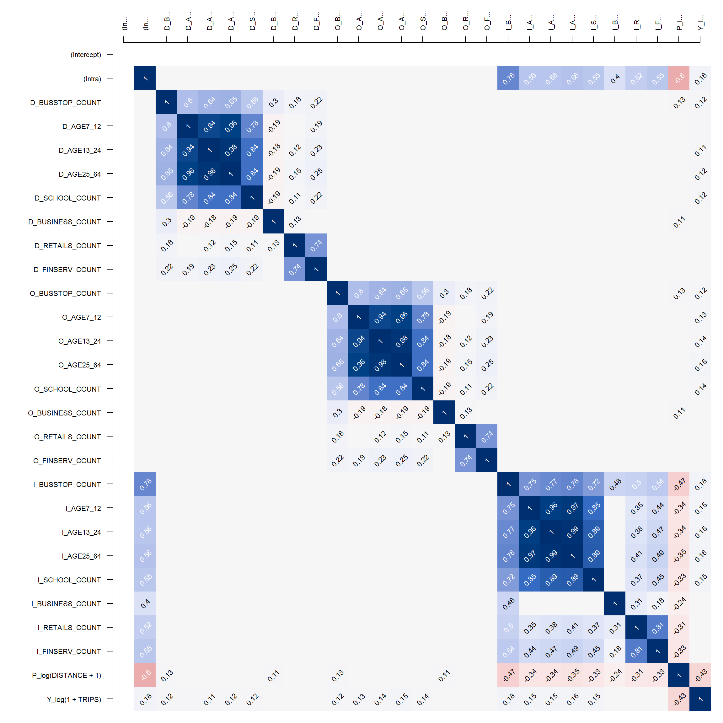
          sg          sg       sg_sg      100.00% 97969/97969 313/313 313/313

Check for Multicollinearity

cor_formula <- log(1 + TRIPS) ~
  BUSSTOP_COUNT + 
  AGE7_12 + 
  AGE13_24 + 
  AGE25_64 + 
  SCHOOL_COUNT + 
  BUSINESS_COUNT + 
  RETAILS_COUNT + 
  FINSERV_COUNT + 
  P_(log(DISTANCE + 1))   # P stands for the impedence

cor_mat <- pair_cor(
  mpsz_multi_net,
  spflow_formula = cor_formula,
  add_lags_x = FALSE
)

# Labels
colnames(cor_mat) <- paste0(substr(colnames(cor_mat),1,3),"...")

cor_image(cor_mat)

Base Model Calibration

There are currently three estimators of spatial econometric interaction models supported by spflow package:

Maximum likelihood estimation (MLE) – default estimation procedure.
Spatial two-stage least squares (S2SLS) – activate the S2SLS estimation via the estimation_control argument using the input spflow_control(estimation_method = "s2sls").
Bayesian Markov Chain Monte Carlo (MCMC) – activate the MCMC estimation via the estimation_control argument using the input spflow_control(estimation_method = "mcmc").

The function offers a formula interface adapted to spatial interaction models, which has the following structure:

Y ~ O_(X1) + D_(X2) + I_(X3) + P_(X4)

O_(…) and D_(…) indicate which variables are used as characteristics of the origins and destinations respectively
I_(…) indicates variables that should be used for the intra-regional parameters
P_(…) declares which variables describe origin-destination pairs, which usually will include a measure of distance (distance decay).

base_model <- spflow(
  spflow_formula = log(1 + TRIPS) ~
    O_(BUSSTOP_COUNT + 
         AGE25_64) + 
    D_(SCHOOL_COUNT + 
         BUSINESS_COUNT + 
         RETAILS_COUNT + 
         FINSERV_COUNT) + 
    P_(log(DISTANCE + 1)),
  spflow_networks = mpsz_multi_net
)

base_model

--------------------------------------------------
Spatial interaction model estimated by: MLE  
Spatial correlation structure: SDM (model_9)
Dependent variable: log(1 + TRIPS)

--------------------------------------------------
Coefficients:
                          est     sd   t.stat  p.val
rho_d                   0.680  0.004  192.554  0.000
rho_o                   0.678  0.004  187.732  0.000
rho_w                  -0.396  0.006  -65.591  0.000
(Intercept)             0.410  0.065    6.266  0.000
(Intra)                 1.313  0.081   16.263  0.000
D_SCHOOL_COUNT          0.017  0.002    7.885  0.000
D_SCHOOL_COUNT.lag1     0.002  0.004    0.551  0.581
D_BUSINESS_COUNT        0.000  0.000    3.015  0.003
D_BUSINESS_COUNT.lag1   0.000  0.000   -0.249  0.804
D_RETAILS_COUNT         0.000  0.000   -0.306  0.759
D_RETAILS_COUNT.lag1    0.000  0.000    0.152  0.880
D_FINSERV_COUNT         0.002  0.000    6.787  0.000
D_FINSERV_COUNT.lag1   -0.002  0.001   -3.767  0.000
O_BUSSTOP_COUNT         0.002  0.000    6.806  0.000
O_BUSSTOP_COUNT.lag1   -0.001  0.000   -2.364  0.018
O_AGE25_64              0.000  0.000    7.336  0.000
O_AGE25_64.lag1         0.000  0.000   -2.797  0.005
P_log(DISTANCE + 1)    -0.050  0.007   -6.793  0.000

--------------------------------------------------
R2_corr: 0.6942944  
Observations: 97969  
Model coherence: Validated

Insights and Interpretation of results

Based on the print result above, model 9 and MLE estimator is used (defaults). The R² value is 0.694, which means the model accounts for 69.42% of the variation of flows.

rho_d - destination constrain rho_o - origin constrain rho_w - intrazonal constrain

D_SCHOOL_COUNT has a t.stat that is statistically significant, but the t.stat of its lag is not statistically significant. Similarly for D_BUSINESS_COUNT and its lag.

School and Business counts in the zone will affect the attractiveness, but not school and business counts in neighbouring zones.

D_RETAILS_COUNT and its lag are both not statistically significant.

Not a good explanatory variable for weekday morning peak.

D_FINSERV_COUNT and its lag are both statistically significant.

Good explanatory variable: Financial services counts in the zone and in neighbouring zones will affect the attractiveness

O_BUSSTOP_COUNT and its lag are both statistically significant. Simialrly for O_AGE25_64 and and its lag.

Good explanatory variable: Financial services counts in the zone and in neighbouring zones will affect the attractiveness

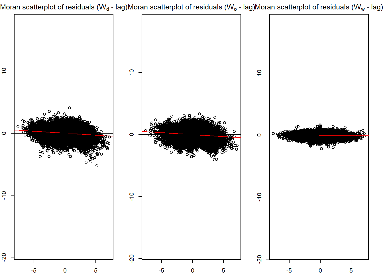
old_par <- par(mfrow = c(1,3),
               mar = c(2,2,2,2))
spflow_moran_plots(base_model)

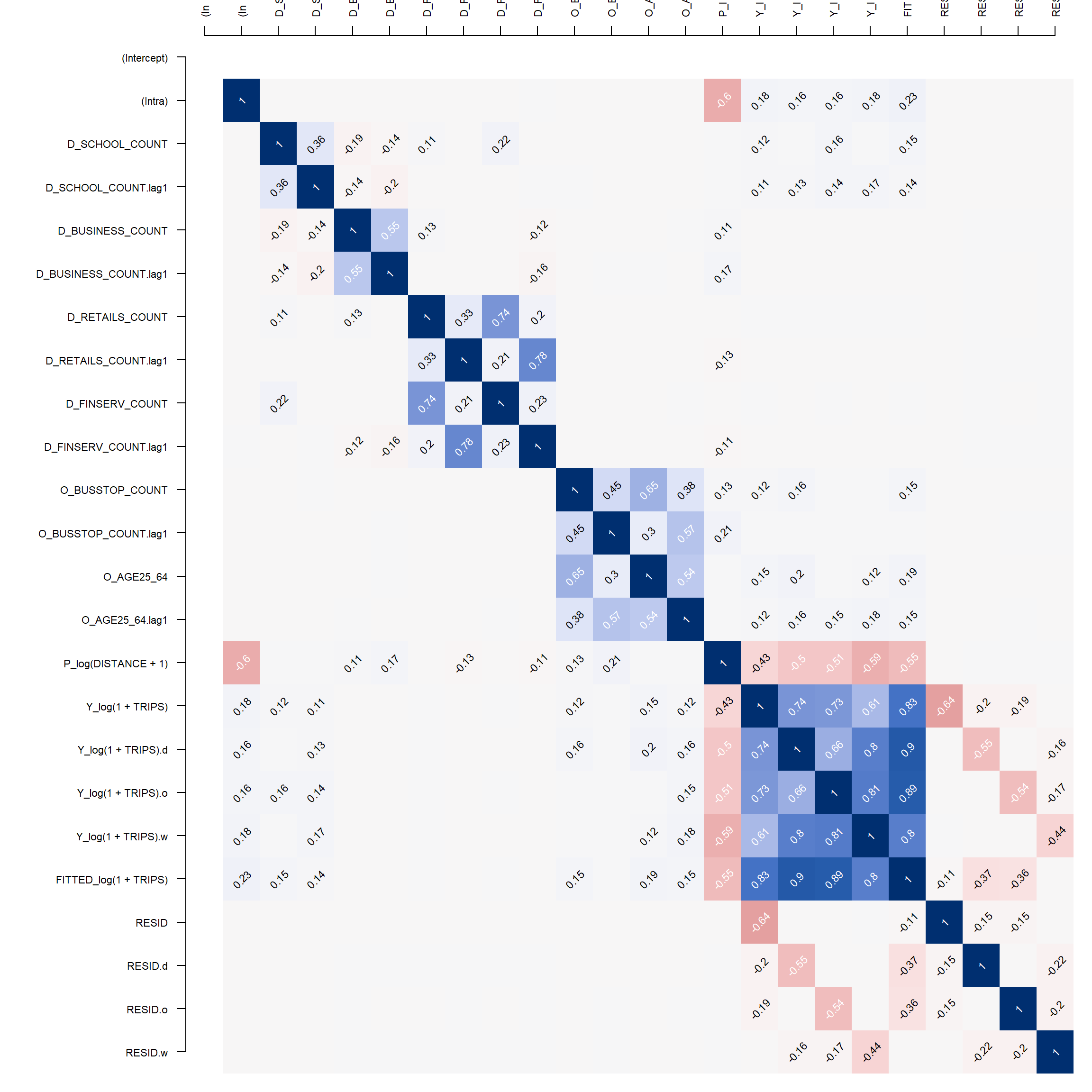
par(old_par)

Next, pair_cor() can be used to inspect the relationship of the residual and the explanatory variables by using the code chunk below.

Check for multi-collinearity again.

corr_residual <- pair_cor(base_model)
colnames(corr_residual) <- substr(colnames(corr_residual),1,3)
cor_image(corr_residual)

Working with model control

Example of running MLE Model 8:

spflow_formula <- log(1 + TRIPS) ~
    O_(BUSSTOP_COUNT + 
         AGE25_64) + 
    D_(SCHOOL_COUNT + 
         BUSINESS_COUNT + 
         RETAILS_COUNT + 
         FINSERV_COUNT) + 
    P_(log(DISTANCE + 1))

model_control <- spflow_control(
  estimation_method = "mle",
  model = "model_8"
)

mle_model8 <- spflow(
  spflow_formula,
  spflow_networks = mpsz_multi_net,
  estimation_control = model_control
)

mle_model8

--------------------------------------------------
Spatial interaction model estimated by: MLE  
Spatial correlation structure: SDM (model_8)
Dependent variable: log(1 + TRIPS)

--------------------------------------------------
Coefficients:
                          est     sd    t.stat  p.val
rho_d                   0.689  0.003   196.832  0.000
rho_o                   0.687  0.004   192.214  0.000
rho_w                  -0.473  0.003  -142.469  0.000
(Intercept)             1.086  0.049    22.275  0.000
(Intra)                 0.840  0.075    11.255  0.000
D_SCHOOL_COUNT          0.019  0.002     8.896  0.000
D_SCHOOL_COUNT.lag1     0.019  0.004     5.130  0.000
D_BUSINESS_COUNT        0.000  0.000     3.328  0.001
D_BUSINESS_COUNT.lag1   0.000  0.000     1.664  0.096
D_RETAILS_COUNT         0.000  0.000    -0.414  0.679
D_RETAILS_COUNT.lag1    0.000  0.000    -0.171  0.864
D_FINSERV_COUNT         0.002  0.000     6.150  0.000
D_FINSERV_COUNT.lag1   -0.003  0.001    -4.601  0.000
O_BUSSTOP_COUNT         0.003  0.000     7.676  0.000
O_BUSSTOP_COUNT.lag1    0.000  0.000     0.552  0.581
O_AGE25_64              0.000  0.000     6.870  0.000
O_AGE25_64.lag1         0.000  0.000    -0.462  0.644
P_log(DISTANCE + 1)    -0.125  0.005   -22.865  0.000

--------------------------------------------------
R2_corr: 0.6965974  
Observations: 97969  
Model coherence: Validated

The R² of Model 8 is 0.696, meaning the model accounts for 69.65% of the variation of flows – slightly higher than that for Model 9.

Example of running MLE Model 1 (unconstrained):

model_control <- spflow_control(
  estimation_method = "mle",
  model = "model_1"
)

mle_model1 <- spflow(
  spflow_formula,
  spflow_networks = mpsz_multi_net,
  estimation_control = model_control
)

mle_model1

--------------------------------------------------
Spatial interaction model estimated by: OLS  
Spatial correlation structure: SLX (model_1)
Dependent variable: log(1 + TRIPS)

--------------------------------------------------
Coefficients:
                          est     sd    t.stat  p.val
(Intercept)            11.384  0.069   164.255  0.000
(Intra)                -6.006  0.112   -53.393  0.000
D_SCHOOL_COUNT          0.093  0.003    28.599  0.000
D_SCHOOL_COUNT.lag1     0.255  0.006    44.905  0.000
D_BUSINESS_COUNT        0.001  0.000    10.036  0.000
D_BUSINESS_COUNT.lag1   0.003  0.000    18.274  0.000
D_RETAILS_COUNT         0.000  0.000    -1.940  0.052
D_RETAILS_COUNT.lag1    0.000  0.000    -2.581  0.010
D_FINSERV_COUNT         0.005  0.000    10.979  0.000
D_FINSERV_COUNT.lag1   -0.016  0.001   -17.134  0.000
O_BUSSTOP_COUNT         0.014  0.001    25.865  0.000
O_BUSSTOP_COUNT.lag1    0.015  0.001    21.728  0.000
O_AGE25_64              0.000  0.000    14.479  0.000
O_AGE25_64.lag1         0.000  0.000    14.452  0.000
P_log(DISTANCE + 1)    -1.281  0.008  -165.327  0.000

--------------------------------------------------
R2_corr: 0.2831458  
Observations: 97969  
Model coherence: Validated

The R² of Model 1 (unconstrained) is only 0.2831, meaning the model accounts for 28.31% of the variation of flows.

Example of running MLE Model 2 (constrained):

model_control <- spflow_control(
  estimation_method = "mle",
  model = "model_2"
)

mle_model2 <- spflow(
  spflow_formula,
  spflow_networks = mpsz_multi_net,
  estimation_control = model_control
)

mle_model2

--------------------------------------------------
Spatial interaction model estimated by: MLE  
Spatial correlation structure: SDM (model_2)
Dependent variable: log(1 + TRIPS)

--------------------------------------------------
Coefficients:
                          est     sd   t.stat  p.val
rho_d                   0.731  0.003  218.603  0.000
(Intercept)             3.068  0.067   45.899  0.000
(Intra)                -0.398  0.093   -4.291  0.000
D_SCHOOL_COUNT          0.063  0.003   24.291  0.000
D_SCHOOL_COUNT.lag1     0.054  0.005   11.802  0.000
D_BUSINESS_COUNT        0.001  0.000    8.790  0.000
D_BUSINESS_COUNT.lag1   0.001  0.000    3.925  0.000
D_RETAILS_COUNT         0.000  0.000   -1.076  0.282
D_RETAILS_COUNT.lag1    0.000  0.000    0.251  0.802
D_FINSERV_COUNT         0.007  0.000   18.054  0.000
D_FINSERV_COUNT.lag1   -0.009  0.001  -12.691  0.000
O_BUSSTOP_COUNT         0.003  0.000    8.269  0.000
O_BUSSTOP_COUNT.lag1    0.004  0.001    7.808  0.000
O_AGE25_64              0.000  0.000    3.918  0.000
O_AGE25_64.lag1         0.000  0.000    4.421  0.000
P_log(DISTANCE + 1)    -0.351  0.007  -47.000  0.000

--------------------------------------------------
R2_corr: 0.5527887  
Observations: 97969  
Model coherence: Validated

The R² of Model 2 (constrained) is 0.5527, meaning the model accounts for 55.27% of the variation of flows – higher than that of Model 1 (unconstrained).