4a: Geocoding

Getting started

The code chunk below uses p_load() of pacman package to check if the required packages have been installed on the computer. If they are, the packages will be launched. The packages used are:

• tmap: for thematic mapping
• sf: for geospatial data wrangling
• tidyverse: for non-spatial data wrangling
• httr: for working with HTTP

pacman::p_load(tmap, sf, httr, tidyverse)

Geocoding using SLA API

Address geocoding, or simply geocoding, is the process of taking a text-based description of a location, such as an address or the name of a place, and returning geographic coordinates, frequently latitude/longitude pair, to identify a location on the Earth’s surface.

SLA supports an online geocoding service called OneMap API. The Search API looks up the address data or 6-digit postal code data and returns a X/Y pair in SVY21 projected coordinate system and a latitude/longitude pair in WGS84 geographical coordinate system.

url <- "https://www.onemap.gov.sg/api/common/elastic/search"

csv <- read_csv("data/aspatial/Generalinformationofschools.csv")
postcodes <- csv$postal_code

found <- data.frame()
not_found <- data.frame()

for (postcode in postcodes) {
  query <- list('searchVal'=postcode, 'returnGeom'='Y', 'getAddrDetails'='Y', 'pageNum'='1')
  res <- GET(url, query=query)
  
  if ((content(res)$found)!=0){
    found <- rbind(found, data.frame(content(res))[4:13])
  } else {
    not_found = data.frame(postcode)
  }
}

Next, the code chunk below will be used to combine both the found and not_found data frames into a single tibble data frame called merged. Additionally, merged and not_found tibble data frames will be written into csv files for future use.

merged <- merge(csv, found, by.x = "postal_code", by.y = "results.POSTAL", all = T)
write_csv(merged, "data/aspatial/schools.csv")
write_csv(not_found, "data/aspatial/not_found.csv")

Next, manually update the csv file for the school where the geocoding could not be completed, then reload the csv file as a schools tibble data frame. A pipe operation is done to rename the coordinates columns and select only required columns.

schools <- read_csv("data/aspatial/schools.csv")

schools <- schools %>%
  rename("latitude" = "results.LATITUDE",
         "longitude" = "results.LONGITUDE") %>%
  select(postal_code, school_name, latitude, longitude)

Converting aspatial data into sf tibble data frame

Next, convert the aspatial data frame into a simple feature tibble data frame called schools_sf using st_as_sf() of sf package. The data frame is then converted into the svy21 projected coordinate system.

Specify the coordinates in the coords argument in the order of longitude followed by latitude.

schools_sf <- st_as_sf(schools, coords = c("longitude", "latitude"), crs = st_crs(4326)) %>%
  st_transform(crs = 3414)

Plotting a point simple feature layer

To ensure that the schools_sf tibble data frame is projected and converted correctly, it will be plotted on a map for visual inspection.

The set.zoom.limits argument ensures that the map cannot be zommed out beyond Singapore and also cannot be zoomed in too much such that the map cannot be loaded.

tmap_mode("view")

tm_shape(schools_sf) +
  tm_dots() + 
  tm_view(set.zoom.limits = c(11,14))

# before moving to the next layer change back to non-interactive mode
tmap_mode("plot") 

Importing geospatial data

Importing Planning and Subzone data

The code chunk below uses the st_read() function of sf package to import MPSZ-2019 shapefile into R as a simple feature data frame called mpsz. To ensure we can use mpsz together with schools_sf, mpsz is reprojected to the svy21 projected coordinate system (crs=3413).

mpsz <- st_read(dsn = "data/geospatial", 
                layer = "MPSZ-2019") %>%
  st_transform(crs=3414)

Reading layer `MPSZ-2019' from data source 
  `C:\magdalenecjw\ISSS624 Geospatial\In_Class_Exercise\Ex4\data\geospatial' 
  using driver `ESRI Shapefile'
Simple feature collection with 332 features and 6 fields
Geometry type: MULTIPOLYGON
Dimension:     XY
Bounding box:  xmin: 103.6057 ymin: 1.158699 xmax: 104.0885 ymax: 1.470775
Geodetic CRS:  WGS 84

The code chunk below counts the number of schools within each planning subzone by using st_intersects() and lengths(), then examines the summary statistics of the new derived variable SCHOOL_COUNT.

mpsz$SCHOOL_COUNT <- lengths(st_intersects(mpsz, schools_sf))

summary(mpsz$SCHOOL_COUNT)

   Min. 1st Qu.  Median    Mean 3rd Qu.    Max. 
  0.000   0.000   0.000   1.054   2.000  12.000 

Importing Planning and Subzone data

biz_sf <- st_read(dsn = "data/geospatial", 
                layer = "Business") %>%
  st_transform(crs=3414)

Reading layer `Business' from data source 
  `C:\magdalenecjw\ISSS624 Geospatial\In_Class_Exercise\Ex4\data\geospatial' 
  using driver `ESRI Shapefile'
Simple feature collection with 6550 features and 3 fields
Geometry type: POINT
Dimension:     XY
Bounding box:  xmin: 3669.148 ymin: 25408.41 xmax: 47034.83 ymax: 50148.54
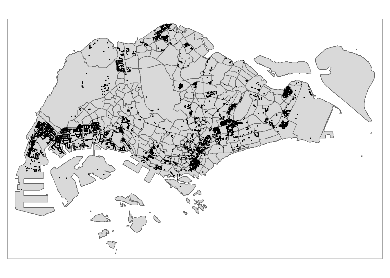
Projected CRS: SVY21 / Singapore TM

To ensure that the biz_sf tibble data frame is projected and converted correctly, it will be plotted on a map for visual inspection.

The check.and.fix argument checks for and fixes geometric errors such as the polygons not being enclosed fully prior to plotting. tm_shape(mpsz) + tm_polygons() provides the boundary map before the biz_sf layer. In order to make use of boundary maps, always plot the polygons first before the points.

tmap_options(check.and.fix = TRUE)
tm_shape(mpsz) +    # boundary map
  tm_polygons() +   # boundary map
  tm_shape(biz_sf) +
  tm_dots()

The code chunk below counts the number of businesses within each planning subzone by using st_intersects() and lengths(), then examines the summary statistics of the new derived variable BIZ_COUNT.

mpsz$BIZ_COUNT <- lengths(st_intersects(mpsz, biz_sf))

summary(mpsz$BIZ_COUNT)

   Min. 1st Qu.  Median    Mean 3rd Qu.    Max. 
   0.00    0.00    2.00   19.73   13.00  307.00