3: Processing and Visualising Flow Data

Author

Magdalene Chan

Published

December 2, 2023

Modified

December 2, 2023

Spatial interaction represents the flow of people, material, or information between locations in geographical space. It encompasses everything from freight shipments, energy flows, and the global trade in rare antiquities, to flight schedules, rush hour woes, and pedestrian foot traffic.

Each spatial interaction is composed of a discrete origin/destination pair. Each pair can be represented as a cell in a matrix where rows are related to the locations (centroids) of origin, while columns are related to locations (centroids) of destination. Such a matrix is commonly known as an origin/destination matrix, or a spatial interaction matrix.

Getting Started

The code chunk below uses p_load() of pacman package to check if the required packages have been installed on the computer. If they are, the packages will be launched.

sf package is used for importing, managing, and processing geospatial data.
tmap package is used for thematic mapping.
tidyverse package is used for importing, integrating, wrangling and visualising data.
stplanr package is used for plotting desire lines on maps.

pacman::p_load(sf, tmap, tidyverse, stplanr, DT)

Preparing Flow Data

Import OD data

Firstly, import the Passenger Volume by Origin Destination Bus Stops data set downloaded from LTA DataMall by using read_csv() of readr package.

odbus <- read_csv("data/aspatial/origin_destination_bus_202310.csv")

Display the odbus tibble data table by using the code chunk below.

glimpse(odbus)

Rows: 5,694,297
Columns: 7
$ YEAR_MONTH          <chr> "2023-10", "2023-10", "2023-10", "2023-10", "2023-…
$ DAY_TYPE            <chr> "WEEKENDS/HOLIDAY", "WEEKDAY", "WEEKENDS/HOLIDAY",…
$ TIME_PER_HOUR       <dbl> 16, 16, 14, 14, 17, 17, 17, 7, 14, 14, 10, 20, 20,…
$ PT_TYPE             <chr> "BUS", "BUS", "BUS", "BUS", "BUS", "BUS", "BUS", "…
$ ORIGIN_PT_CODE      <chr> "04168", "04168", "80119", "80119", "44069", "2028…
$ DESTINATION_PT_CODE <chr> "10051", "10051", "90079", "90079", "17229", "2014…
$ TOTAL_TRIPS         <dbl> 3, 5, 3, 5, 4, 1, 24, 2, 1, 7, 3, 2, 5, 1, 1, 1, 1…

A quick check of odbus tibble data frame shows that the values in ORIGIN_PT_CODE and DESTINATON_PT_CODE are in numeric data type. Hence, the code chunk below is used to convert these data values into character data type.

odbus$ORIGIN_PT_CODE <- as.factor(odbus$ORIGIN_PT_CODE)
odbus$DESTINATION_PT_CODE <- as.factor(odbus$DESTINATION_PT_CODE)

Extract commuting flow data

The code chunk below extracts the commuting flows on weekdays between 6 and 9 o’clock.

odbus6_9 <- odbus %>%
  filter(DAY_TYPE == "WEEKDAY") %>%
  filter(TIME_PER_HOUR >= 6 &
           TIME_PER_HOUR <= 9) %>%
  group_by(ORIGIN_PT_CODE,
           DESTINATION_PT_CODE) %>%
  summarise(TRIPS = sum(TOTAL_TRIPS))

The table below shows the content of odbus6_9

datatable(odbus6_9)

The output is saved in rds format for future use.

write_rds(odbus6_9, "data/rds/odbus6_9.rds")

The code chunk below will be used to import the saved odbus6_9.rds into R environment.

odbus6_9 <- read_rds("data/rds/odbus6_9.rds")

Working with Geospatial data

For this exercise, two geospatial data will be used:

BusStop: This data provides the location of bus stop as at last quarter of 2022.
MPSZ-2019: This data provides the sub-zone boundary of URA Master Plan 2019.

Both data sets are in ESRI shapefile format.

Import geospatial data

The two code chunks below are used to import both sets of geospatial data.

st_read() function of sf package is used to import the shapefile into R as sf data frame. st_transform() function of sf package is used to transform the projection to crs 3414.

BusStop <- st_read(dsn = "data/geospatial", layer = "BusStop") %>%
  st_transform(crs = 3414)

Reading layer `BusStop' from data source 
  `C:\magdalenecjw\ISSS624 Geospatial\Hands_on_Exercise\Ex3\data\geospatial' 
  using driver `ESRI Shapefile'
Simple feature collection with 5161 features and 3 fields
Geometry type: POINT
Dimension:     XY
Bounding box:  xmin: 3970.122 ymin: 26482.1 xmax: 48284.56 ymax: 52983.82
Projected CRS: SVY21

mpsz <- st_read(dsn = "data/geospatial", layer = "MPSZ-2019") %>%
  st_transform(crs = 3414)

Reading layer `MPSZ-2019' from data source 
  `C:\magdalenecjw\ISSS624 Geospatial\Hands_on_Exercise\Ex3\data\geospatial' 
  using driver `ESRI Shapefile'
Simple feature collection with 332 features and 6 fields
Geometry type: MULTIPOLYGON
Dimension:     XY
Bounding box:  xmin: 103.6057 ymin: 1.158699 xmax: 104.0885 ymax: 1.470775
Geodetic CRS:  WGS 84

The code chunk below will be used to write the mpsz sf tibble data frame into an rds file for future use.

mpsz <- write_rds(mpsz, "data/rds/mpsz.rds")

Geospatial Data Wrangling

The code chunk below populates the planning subzone code (i.e. SUBZONE_C) of mpsz sf data frame into busstop sf data frame.

st_intersection() is used to perform point and polygon overlay and the output will be in point sf object. select() of dplyr package is then use to retain only BUS_STOP_N and SUBZONE_C in the busstop_mpsz sf data frame. Five bus stops are excluded in the resultant data frame as they are outside of Singapore’s boundary.

busstop_mpsz <- st_intersection(BusStop, mpsz) %>%
  select(BUS_STOP_N, SUBZONE_C) %>%
  st_drop_geometry()

datatable(busstop_mpsz)

Before moving to the next step, save the output into rds format.

write_rds(busstop_mpsz, "data/rds/busstop_mpsz.rds")

Next, append the planning subzone code from busstop_mpsz data frame onto odbus6_9 data frame.

od_data <- left_join(odbus6_9 , busstop_mpsz,
            by = c("ORIGIN_PT_CODE" = "BUS_STOP_N")) %>%
  rename(ORIGIN_BS = ORIGIN_PT_CODE,
         ORIGIN_SZ = SUBZONE_C,
         DESTIN_BS = DESTINATION_PT_CODE)

It is good practice to check for duplicating records before continuing further with the data wrangling.

duplicate <- od_data %>%
  group_by_all() %>%
  filter(n()>1) %>%
  ungroup()

duplicate

# A tibble: 1,186 × 4
   ORIGIN_BS DESTIN_BS TRIPS ORIGIN_SZ
   <chr>     <fct>     <dbl> <chr>    
 1 11009     01341         1 QTSZ01   
 2 11009     01341         1 QTSZ01   
 3 11009     01411         4 QTSZ01   
 4 11009     01411         4 QTSZ01   
 5 11009     01421        17 QTSZ01   
 6 11009     01421        17 QTSZ01   
 7 11009     01511        19 QTSZ01   
 8 11009     01511        19 QTSZ01   
 9 11009     01521         2 QTSZ01   
10 11009     01521         2 QTSZ01   
# … with 1,176 more rows

As there duplicated records found, the code chunk below will be used to retain the unique records.

od_data <- unique(od_data)

Check that the duplicating records issue has now been resolved.

duplicate <- od_data %>%
  group_by_all() %>%
  filter(n()>1) %>%
  ungroup()

duplicate

# A tibble: 0 × 4
# … with 4 variables: ORIGIN_BS <chr>, DESTIN_BS <fct>, TRIPS <dbl>,
#   ORIGIN_SZ <chr>

Next, update the od_data data frame with the planning subzone codes.

od_data <- left_join(od_data , busstop_mpsz,
            by = c("DESTIN_BS" = "BUS_STOP_N"))

Again, check for duplicates and retain unique records.

Show code

duplicate <- od_data %>%
  group_by_all() %>%
  filter(n()>1) %>%
  ungroup()

od_data <- unique(od_data)

od_data <- od_data %>%
  rename(DESTIN_SZ = SUBZONE_C) %>%
  drop_na() %>%
  group_by(ORIGIN_SZ, DESTIN_SZ) %>%
  summarise(MORNING_PEAK = sum(TRIPS))

Save the output into an rds file format.

write_rds(od_data, "data/rds/od_data.rds")

od_data <- read_rds("data/rds/od_data.rds")

Visualising Spatial Interaction

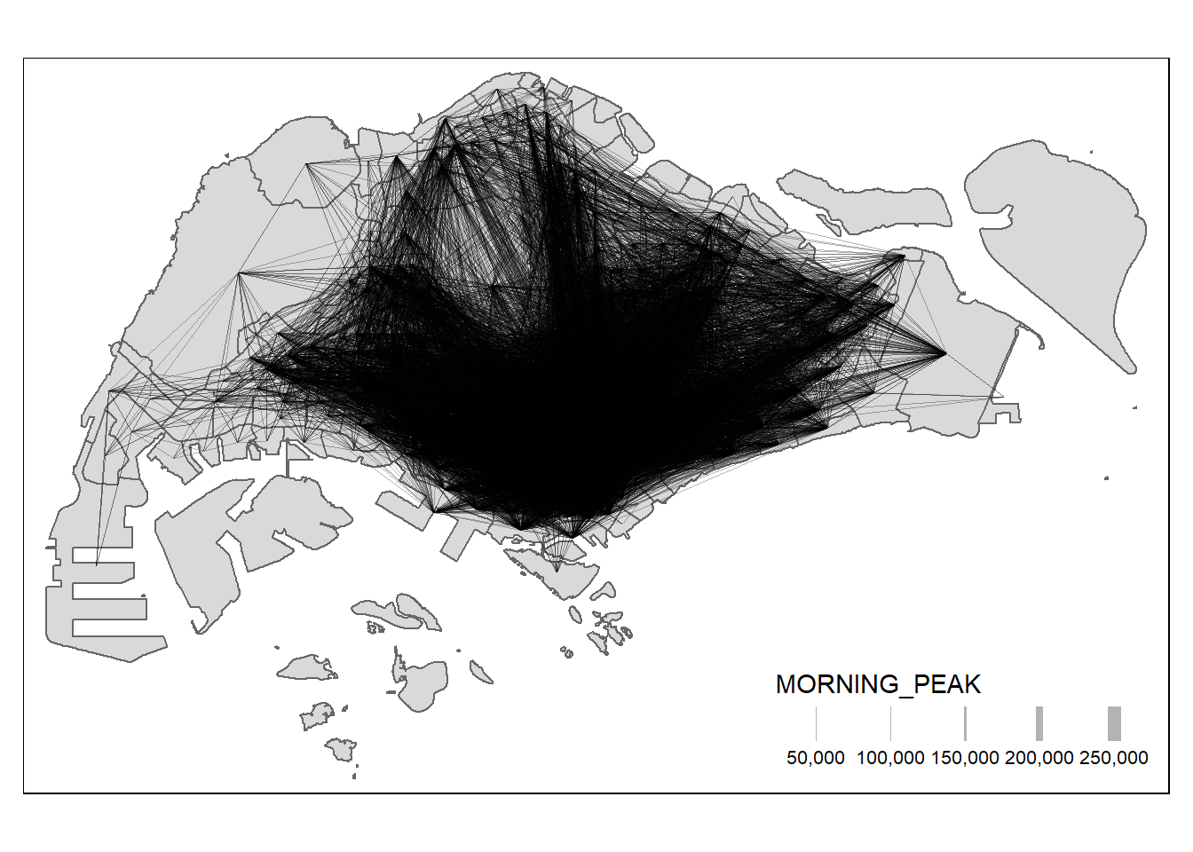
Desire lines are rays connecting a site to associated location points. This section details the steps to prepare a desire line using the stplanr package.

Remove intra-zonal flows

The code chunk below will be used to remove intra-zonal flows which will not be plotted.

od_data1 <- od_data[od_data$ORIGIN_SZ!=od_data$DESTIN_SZ,]

Create desire lines

In this code chunk below, od2line() of stplanr package is used to create the desire lines.

flowLine <- od2line(flow = od_data1, 
                    zones = mpsz,
                    zone_code = "SUBZONE_C")

Visualise desire lines

To visualise the resulting desire lines, the code chunk below is used. > Rendering may take longer due to the transparency argument i.e. alpha.

tm_shape(mpsz) +
  tm_polygons() +
flowLine %>%  
tm_shape() +
  tm_lines(lwd = "MORNING_PEAK",
           style = "quantile",
           scale = c(0.1, 1, 3, 5, 7, 10),
           n = 6,
           alpha = 0.3)

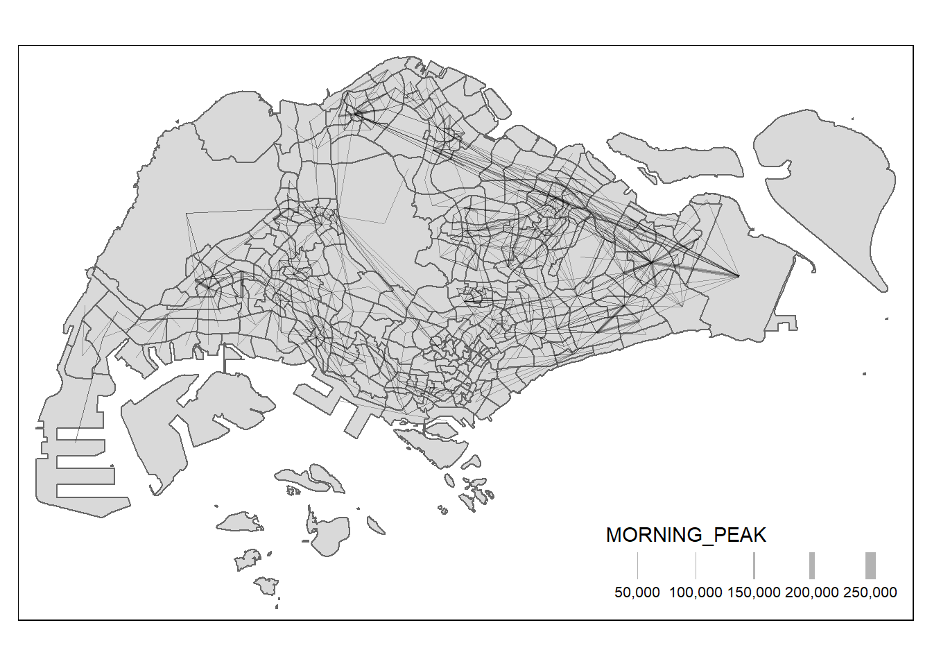
In the chart above, the flow data is very messy and highly skewed. As such, it may be better to focus on selected flows, such as flows greater than or equal to 5000 as shown below.

tm_shape(mpsz) +
  tm_polygons() +
flowLine %>%  
  filter(MORNING_PEAK >= 5000) %>%
tm_shape() +
  tm_lines(lwd = "MORNING_PEAK",
           style = "quantile",
           scale = c(0.1, 1, 3, 5, 7, 10),
           n = 6,
           alpha = 0.3)